AutoML - Time Series Model
A Time series model is a supervised machine learning technique that analyzes sequential data collected over time to identify patterns, trends, and seasonality, and uses them to forecast future values.
- Sales Forecasting: Predict future sales by analyzing historical sales data, helping businesses plan inventory, production, and sales strategies.
- Website Traffic Prediction: Predict future website visits using historical traffic patterns to support capacity planning, marketing campaigns, and resource allocation.
- Stock Price Prediction: Analyze historical stock market data to identify trends and estimate future stock prices or market movements.
Access to AutoML
Roles with administrator privileges, such as Account Admin, Org Admin, Workspace Admin, and users with custom permission, can build ML models.
Build a Time Series Model in Zoho Analytics
Build a time series model in Zoho Analytics comprises of 4 steps.
- Invoke AutoML
- Choose Model Type & Configurations
- Train and Validate the Model
- Deploy the ML Model
- Interpret Results
Invoke AutoML
- Click AutoML from the side navigation panel.
- Click Create New Analysis.
- Choose Build From Scratch.
Choose Model Type
- Choose the ML model as Time Series model.
- In the select configurations section,
- Training Table: Select the training table that should be used for training the model. The model uses this data to learn the relationship between predictor variables and the target variable before making predictions on new data.
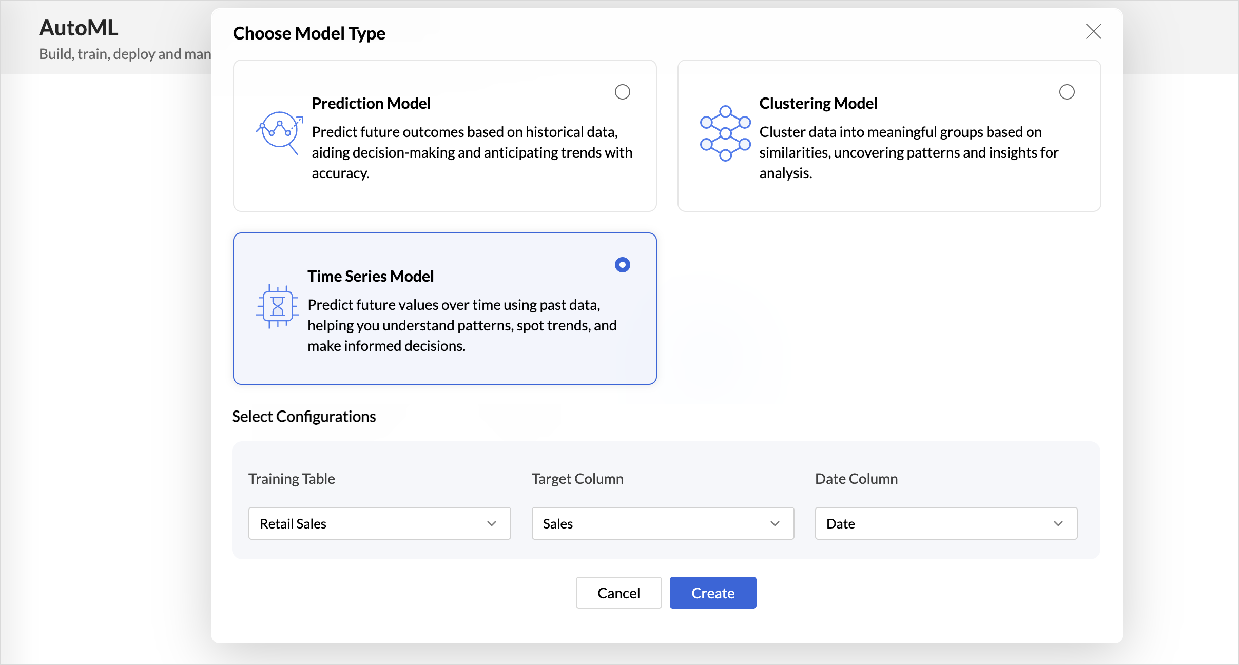
- Training Table: Select the training table that should be used for training the model. The model uses this data to learn the relationship between predictor variables and the target variable before making predictions on new data.
- Click Create.
Time Series Model Configurations
This section lets you configure model-specific settings, including data settings, the algorithm, and feature selection. By default, these settings are automatically configured, but you can customize them to suit your requirements.
- General Settings: Provide a meaningful Name and Description for the prediction model to help identify and manage it later.
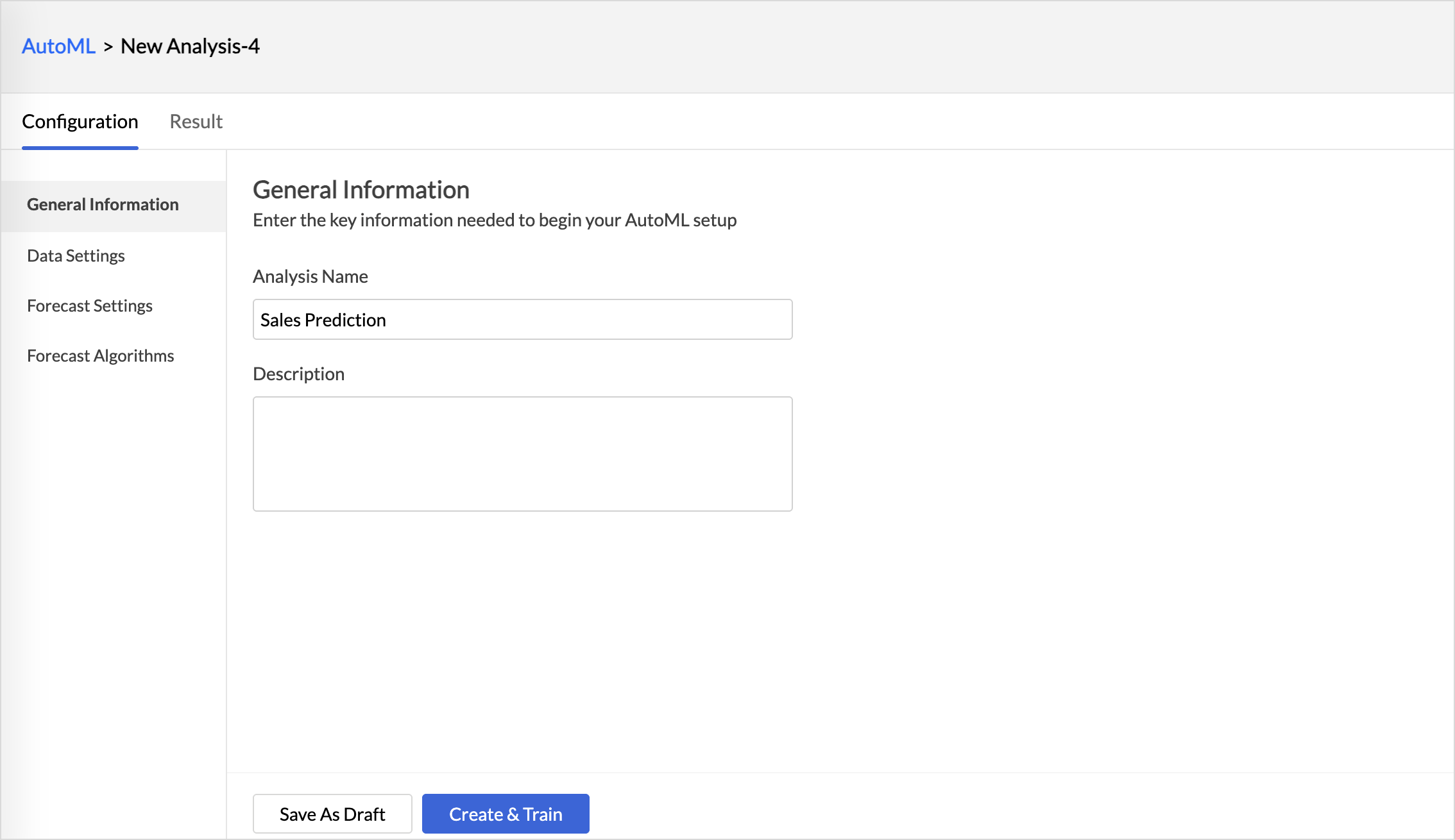
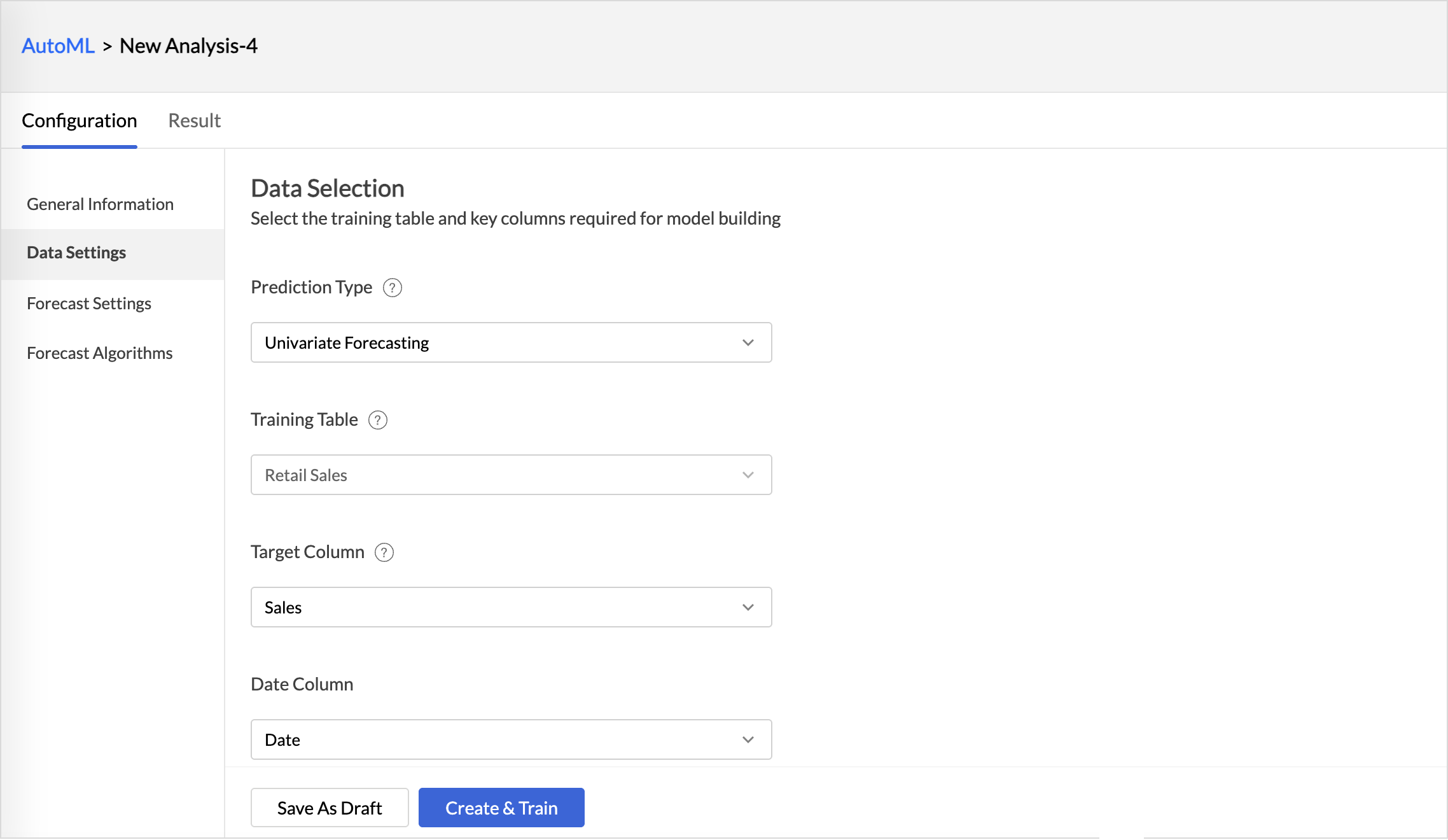
- Data Settings: Choose the Prediction Type based on the target variable you want to predict.
- Uni-variate: Predicts future values based on the historical data of a single time-series variable. It is best suited for scenarios where the forecast depends only on the past values of the target variable, without considering external factors.
- MultiVariate: Predicts future values by analyzing the historical data of the target variable along with one or more related variables (features). It is ideal for scenarios where external factors influence the target variable, resulting in more accurate and context-aware forecasts.
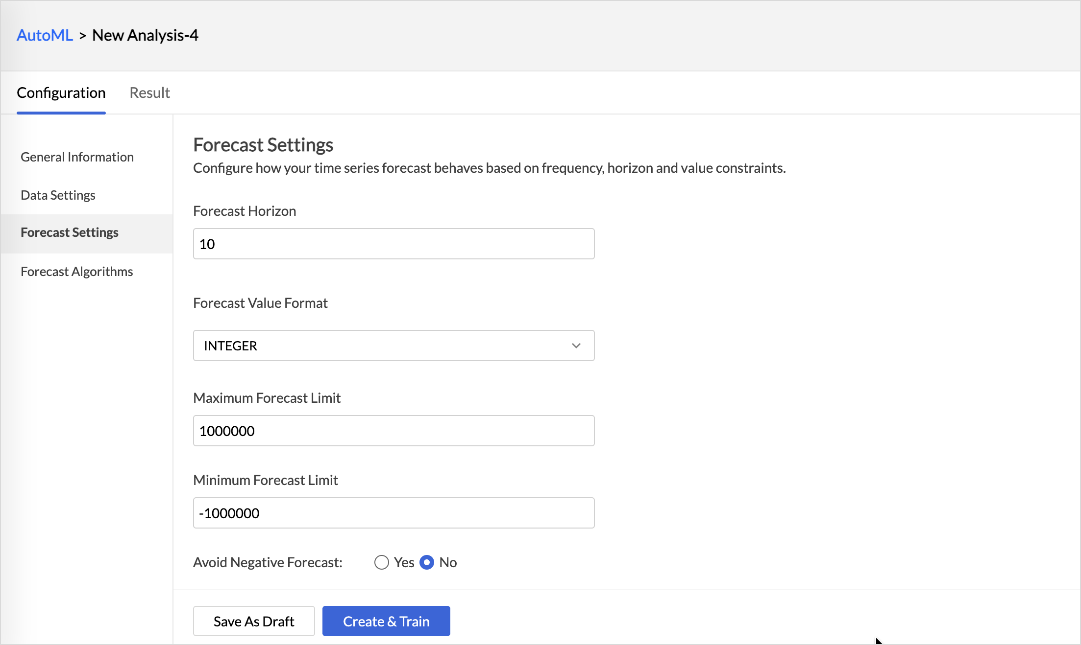
- Forecast Settings: Configure how your time series forecast behaves based on frequency, horizon and value constraints.
- Forecast Horizon: Specify the number of future data points to predict.
- Forecast Format: Choose the format in which the forecasted results should be generated.
- Maximum and Minimum Forecast Limit: Set the lower and upper limit for forecasted values to ensure predictions do not fall below a specified threshold.
- Avoid Negative Forecast: Specify whether to prevent the model from generating negative forecast values.
- Prediction Algorithms: By default, Zoho Analytics automatically selects the most suitable algorithms for model training. To use specific algorithms, enable the toggle switch and choose the algorithms you want AutoML to use during training.
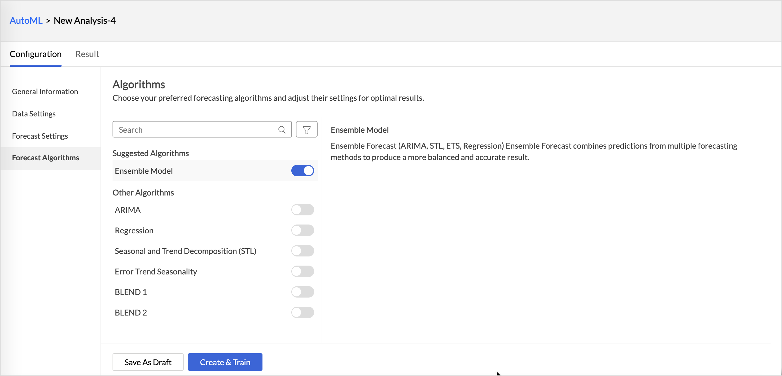
- Save as Draft: Click Save as Draft to save the current model configuration without starting the training process. This preserves all configured settings, including the selected algorithms and features, allowing you to review or modify the configuration before training.
- Create and Train: Click Create and Train to proceed to the model training configuration.The Save as Draft option lets you preserve the model configuration, including algorithm selection and feature settings, so that you can initiate model training later at your convenience.
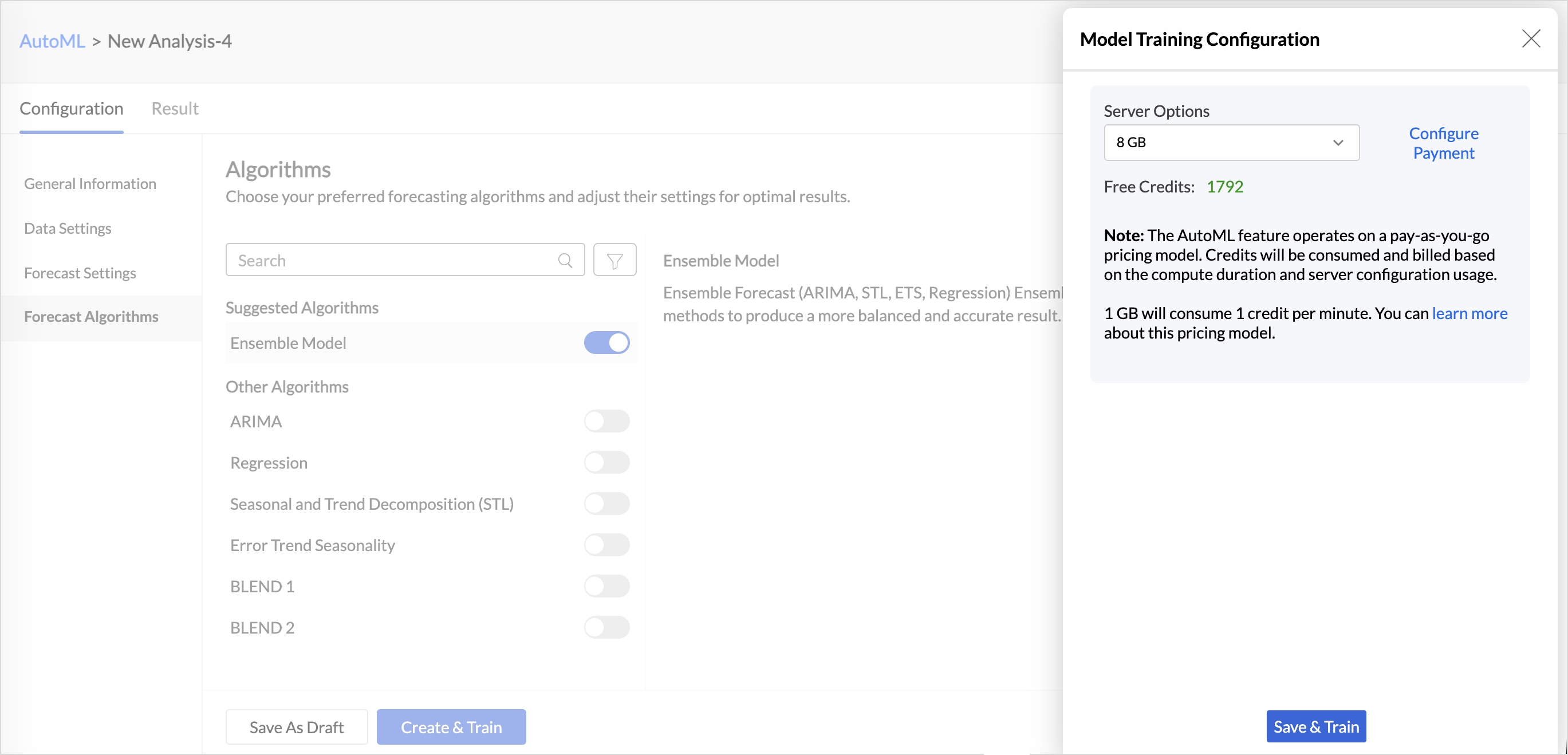
- Model Training Configuration: Choose the Server options for training the ML model. Available server options 8GB, 16GB, 32GB and 128GB.
Train and Validate the ML Model
Once the training is complete, a result tab will be provided to know about the performance and accuracy of each algorithm that was used for training. The Results tab will give an overview of each model's performance, such as the Model Score, Training Status, Trained on, Deployment Status, and Deployment Time.
Select the specific model to get a detailed summary about the performance of the training model. The model details and explanation and performance are specific to each algorithm selected for training.
Model Details
The Model Details tab will list the Model Summary, Algorithm Details, and the Training Details.

Performance
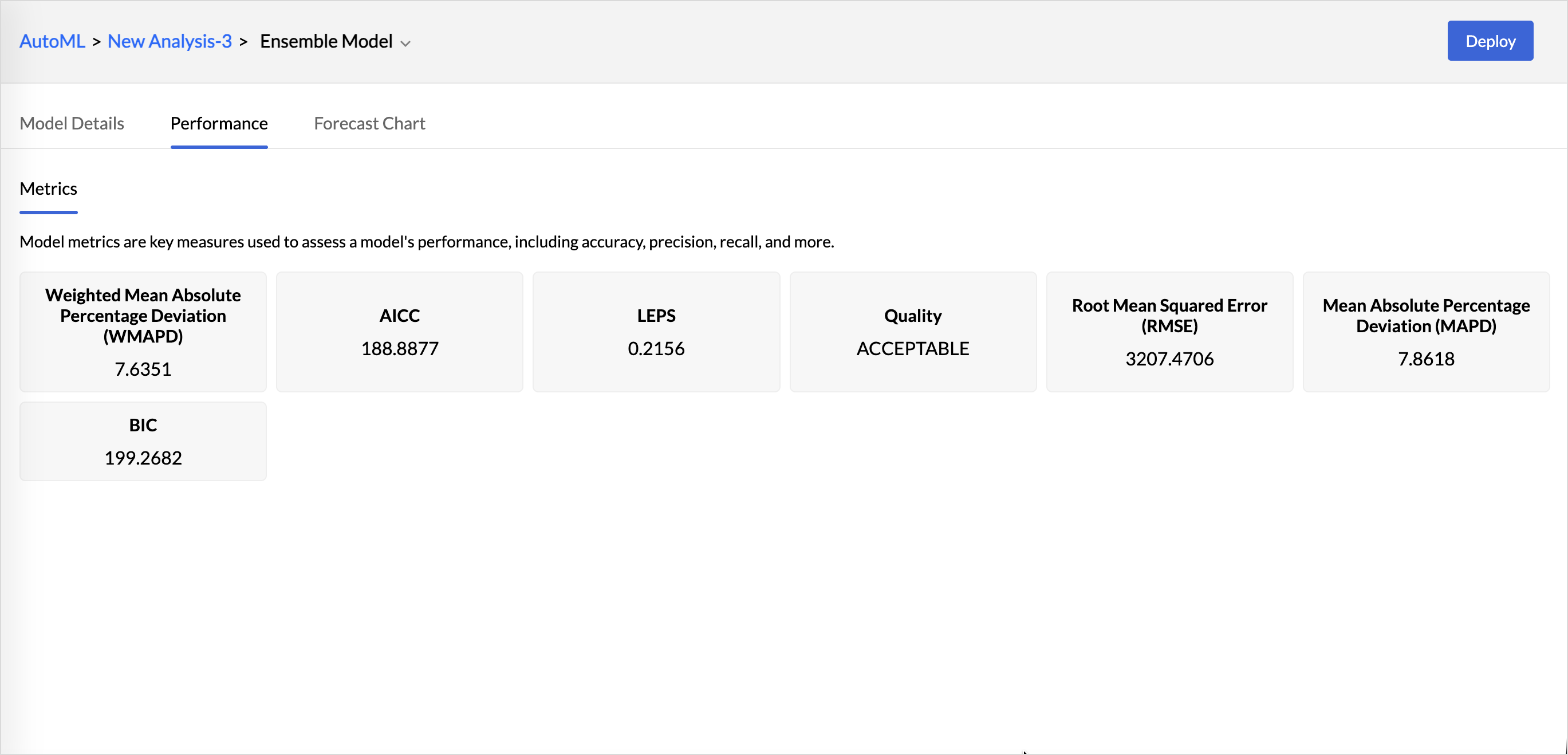
This section lists the metrics, all the statistical measures used to evaluate the accuracy and precision of the ML model. Metrics are the key measures that are used for evaluating the model's performance.
- Weighted Mean Absolute Deviation: Measures the weighted average percentage difference between actual and predicted values. Lower values indicate better forecast accuracy.
- AICC (Corrected Akaike Information Criterion): Evaluates the quality of the model while accounting for the number of parameters and sample size. Lower values indicate a better-fitting model.
- LEPS ( Linear Error in Probability Space): Measures forecast accuracy by comparing predicted and actual values in probability space. Lower values indicate more accurate predictions.
- Root Mean Squared Error: Measures the average magnitude of prediction errors, giving greater weight to larger errors. Lower values indicate better model performance.
- Mean Absolute Percentage Error: Measures the weighted average percentage difference between actual and predicted values. Lower values indicate better forecast accuracy.
- BIC (Bayesian Information Criterion): Evaluates model quality by balancing goodness of fit with model complexity. Lower values indicate a better trade-off between accuracy and complexity.
Forecast Chart
Forecast charts visualize projected trends of target metric with associated confidence intervals.

Deploy ML Model
Once you have assessed the quality and fine-tuned the ML model, you can deploy it on a production dataset to which the trained model should be deployed.
Zoho Analytics allows you to deploy the model in the following two ways:
- Access the Results tab and click the Deploy option adjacent to the model name.
- Access the More Details page and click the Deploy option in the top right corner.
Input Details
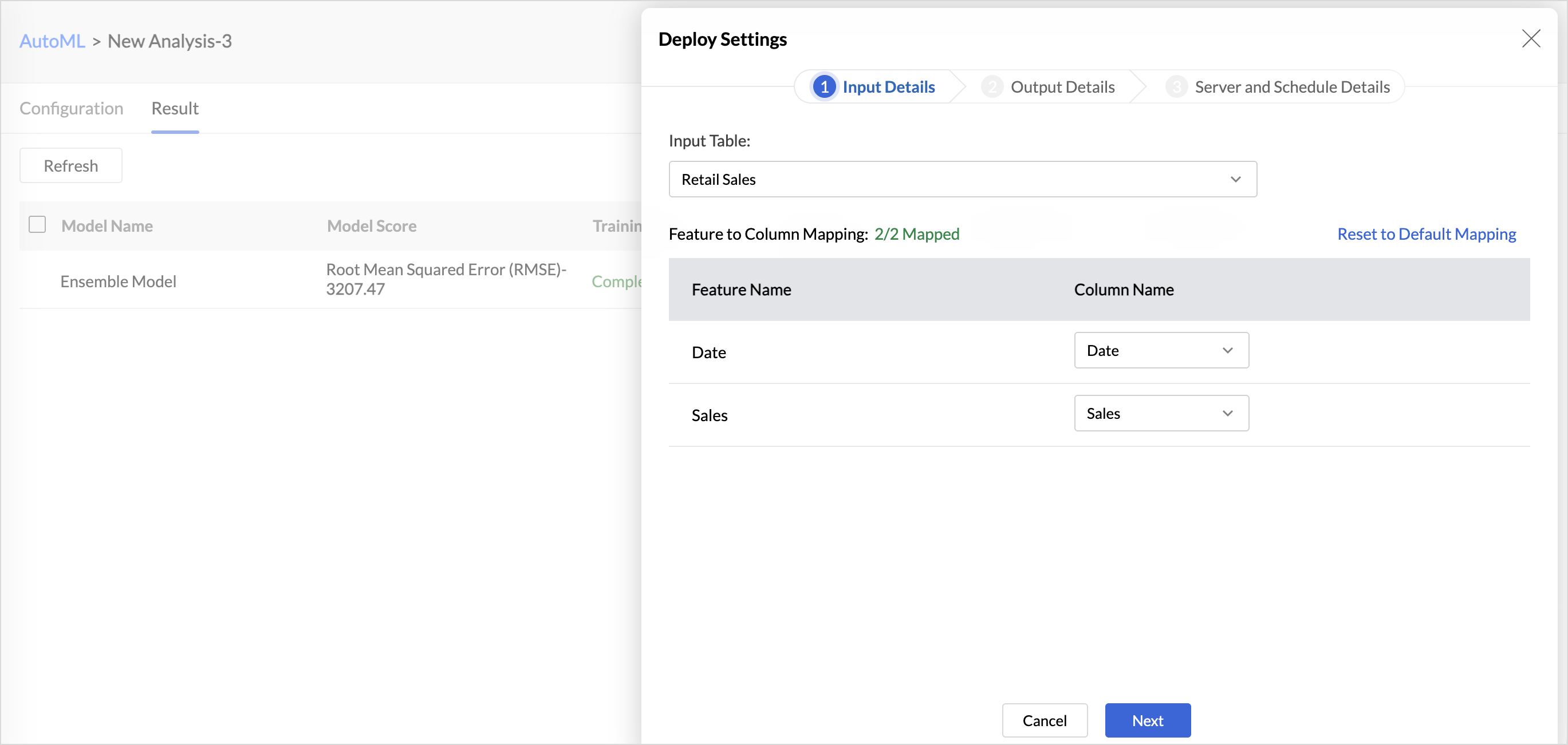
Select the table containing the data on which the trained model will be applied. During deployment, the model processes each record in this table and generates the corresponding prediction or classification result.
- Input Table: Choose the table that contains the data to be scored by the trained model.
- Features (Columns): Select the columns that should be used as input features for generating predictions.
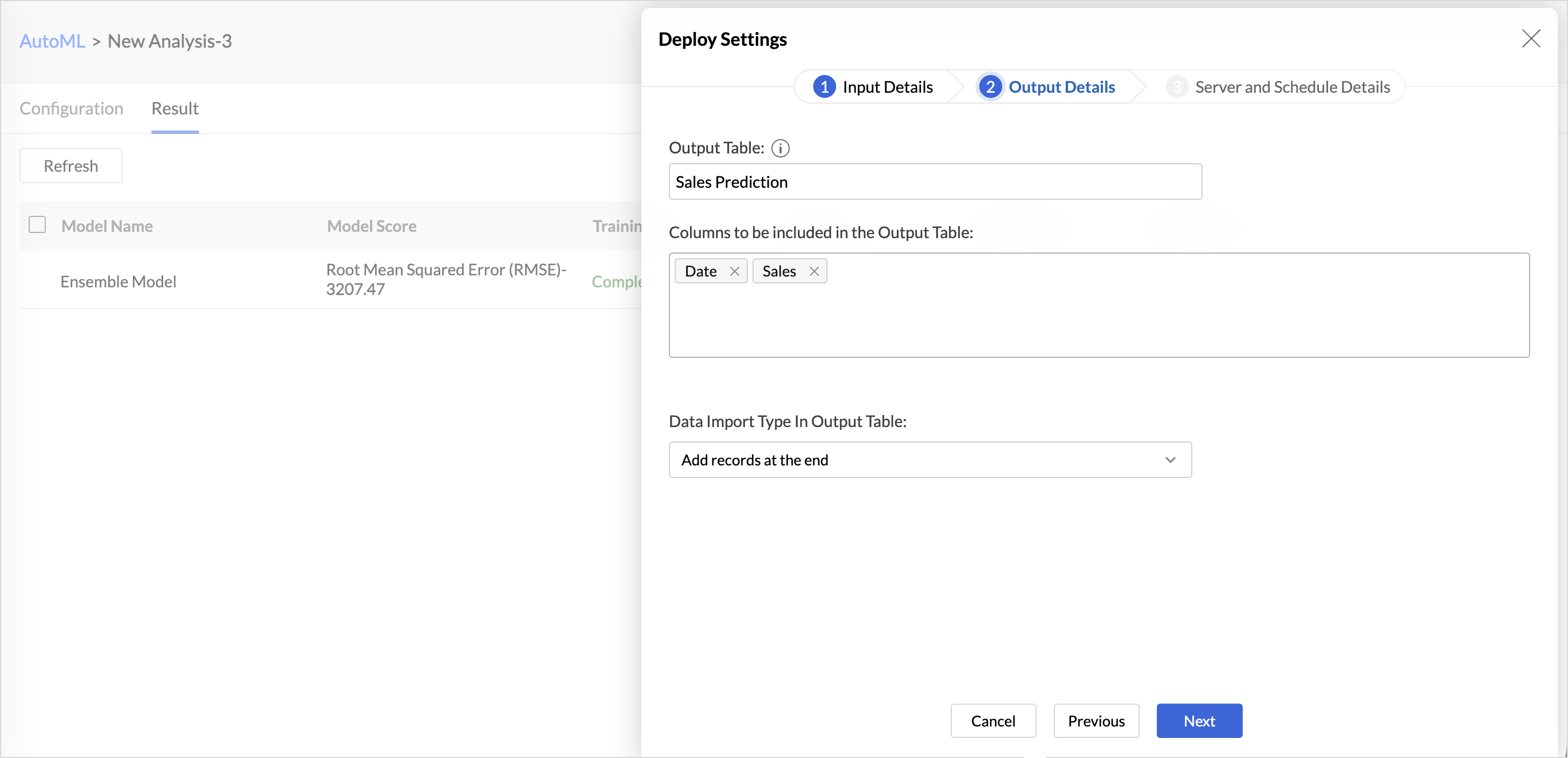
Output Details
- Output Table Name: Enter a suitable name for the output table.The output table is created during the initial deployment. If a schedule is configured, the model is automatically applied to new data added to the source table, and the prediction results are written to this output table.
- Columns to Include: Select the columns from the input table that should be retained in the output table along with the generated prediction results. This helps preserve the relevant business context for each scored record.
- Data Import Type: Choose how the generated prediction records should be written to the output table during each deployment run.
Server and Schedule Details
- Server Option: Select the server configuration that should be used for deployment. Refer to the Pricing Plan section for details about available server options and resource usage.
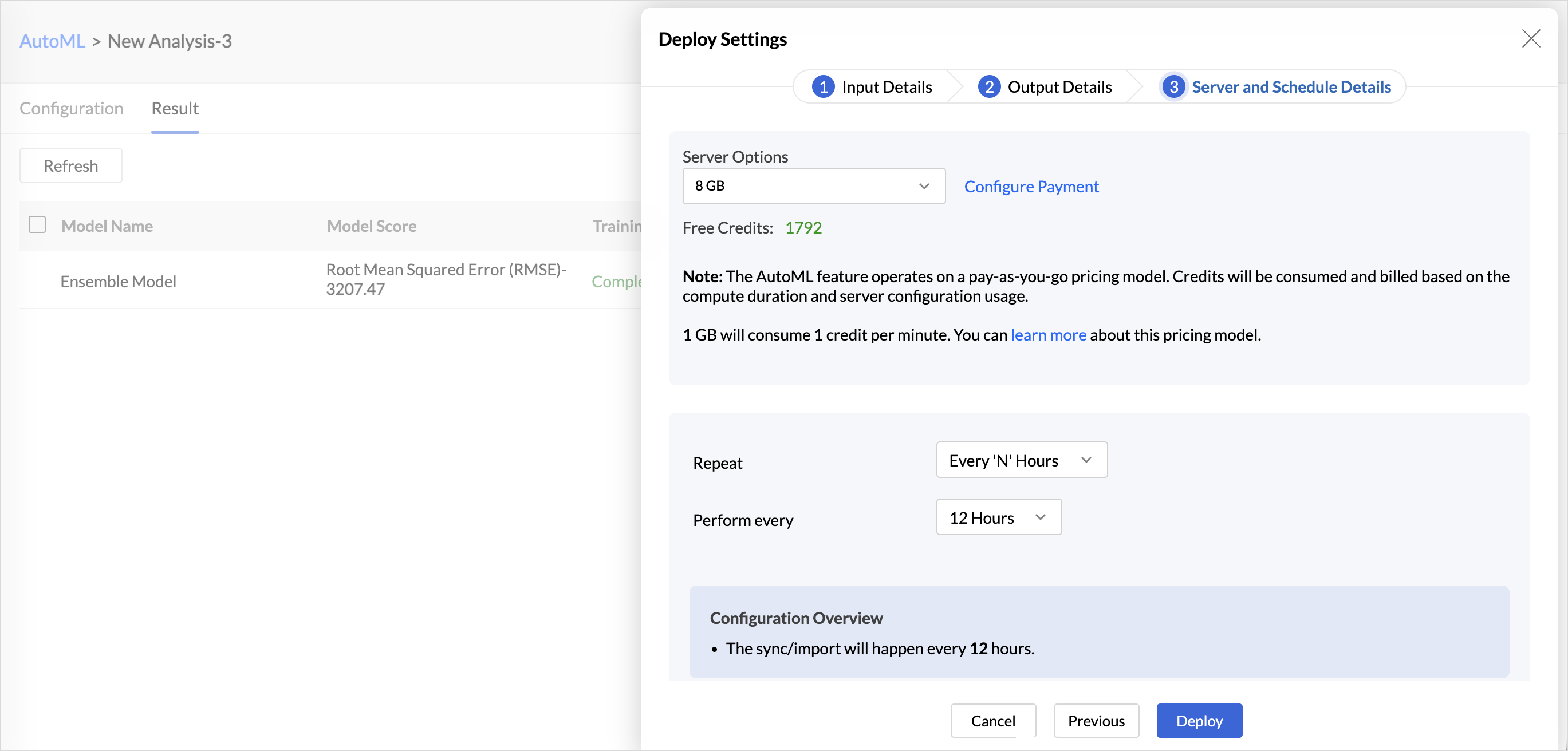
- Repeat: This option allows you to periodically apply the trained model results to the newly added data in the chosen input table. Choose the frequency in which the data should be added to the input table. Available options are:
- Every N Hours
- Every Day
- Weekly Once
- Monthly Once
Time Series Algorithms
Time Series algorithms are statistical and machine learning techniques used to analyse historical time-based data, identify patterns such as trends and seasonality, and forecast future values. AutoML evaluates different forecasting approaches to select the most suitable model based on the characteristics of your data.
Ensemble Model
Combines predictions from multiple forecasting models to generate a single, more accurate and robust forecast. By leveraging the strengths of different models, ensemble forecasting often improves prediction accuracy and reduces the impact of individual model limitations.
ARIMA (AutoRegressive Integrated Moving Average)
ARIMA, a statistical forecasting model that predicts future values by analyzing historical patterns, trends, and auto correlations in a single time-series. It is well suited for univariate forecasting and performs best when the data exhibits consistent temporal patterns after being made stationary.
| Parameter | Description | Default Value |
| Differencing Order | Specifies the number of times the time series is differenced to make it stationary. | 0 |
| AutoRegressive Order | Denotes the number of previous observations used to predict future values | 0 |
| Moving Average Order | Denotes the number of previous forecasts errors used to improve predictions | 0 |
| Max Differencing Order | Sets the maximum differencing order that AutoML can evaluate while selecting the best ARIMA model. | 0 |
| Max Autoregressive Order | Sets the maximum autoregressive order (p) that AutoML can evaluate during model selection. | 0 |
| Max Moving Average Order | Sets the maximum moving average order (q) that AutoML can evaluate during model selection. | 0 |
| Include Constant Terms | Determines whether the model should include a constant term while training. A constant term helps capture the baseline level or average value of the time series when there is no trend component. | Yes |
| Apply Log Transformation | Specifies whether a logarithmic transformation should be applied to the target variable before training. This helps stabilize variance and can improve forecasting performance when the data shows exponential growth or large fluctuations. | No |
Regression
A forecasting approach that predicts continuous future values by learning the relationship between a target variable and one or more input variables (features). It is best suited for multivariate forecasting, where external factors influence the target variable.
| Parameter | Description | Default Value |
| Degree of the Polynomial | Specifies the degree of the polynomial used to model non-linear relationships between the input variables and the target variable. A value of 1 represents linear regression. | 0 |
| Exclude Intercept | Specifies whether to exclude the intercept (constant term) from the regression model. Enable this option only if the relationship is expected to pass through the origin. | Yes |
| Regression Model Type | Specifies the type of regression model to use for forecasting. Choose a model based on the complexity of your data and the relationship between the input variables and the target variable. | Linear |
Seasonal Trend Decomposition
Seasonal Trend Decomposition forecasting is a technique that decomposes a time series into three components trend, seasonality, and residual to understand underlying patterns better and generate more accurate forecasts. It is useful for data with recurring seasonal patterns and long-term trends.
| Parameter | Description | Default Value |
| STL Model Type | Specifies the type of Seasonal and Trend Decomposition model used for forecasting.
|
Error Trend Seasonality
Error Trend Seasonality forecasts future values by modeling the error, trend, and seasonal components of a time series. It is best suited for data with recurring seasonal patterns and long-term trends.
| Parameter | Description | Default Value |
| Level Smoothing | Controls how much weight is given to the most recent observations when estimating the current level of the time series. Higher values make the model respond more quickly to recent changes, while lower values produce smoother forecasts. | 0 |
| ETS Model Type | Determines the type of Exponential Smoothing model used for forecasting. The selected model defines how the algorithm handles the level, trend, and seasonality components of the time series. | Simple_ES |
Blend 1
Combines the predictions from the top-performing single model with another model or forecasting approach to create a blended prediction. It provides a simple ensemble that balances the strengths of different models.