Customizing a Pivot Table

When designing a Pivot Table, the Zoho Advanced Analytics app offers a wide range of options to customize it and improve the overall appearance in different ways. 

In this section, we will discuss various options provided by Zoho Advanced Analytics to customize the Pivot Table.

• Customizing with Pivot Table Settings
  • Title, Description, and Show Missing Values
  • Format 
  • Layout
• Show/Hide
• Show Total As
• Sorting a Pivot Table
• Conditional Formatting
• Applying Themes

Customizing with Pivot Table Settings 

Zoho Advanced Analytics offers options to personalize the look and feel of your Pivot Table. You can customize the various elements in the Pivot (hide row numbers, wrap text in header, etc.,) and personalize them based on your needs.

To customize the appearance of the Pivot, 

1. Open the Pivot Table you would like to customize.
2. Select the Settings option in the toolbar. This will open up the Settings dialog box. You will notice that this dialog contains three tabs -General, Format, and Layout.

Title, Description, and Show Missing Values

Zoho Advanced Analytics provides options to modify the title, description, and data - display in theGeneral tab of your Pivot Table. 

Title and Description: Here you can edit the Title and Descriptionof the Pivot Table.

• Title: You can edit the title of your Pivot Table from here. This field is mandatory.
• Description: You can change the description of your Pivot Table from here. This field is optional.

Show Missing Values: You can choose to display the filtered values from here.

• For columns in the 'Columns' shelf: You can choose to display the filtered columns in the 'Columns' shelf by selecting/deselecting the check box. By default, this value will not be selected.
  To learn more about missing values, refer the below section.
• For columns in the 'Rows' shelf: You can choose to display the filtered columns in the 'Rows' shelf by selecting/deselecting the check box. By default, this value will not be selected. 
  To learn more about missing values, refer the below section.

Show Missing Values

Show missing values feature is used to display the in-between missing values in a Pivot. This can be applied on a Date or a Category column. When creating a Pivot, if a particular data point does not have any value, then the Pivot would skip displaying that data. With this option, you can choose to display the record even if a point does not contain a value. 

Let us say that you want to check the find out the days without any orders. 

Let's now create a pivot as shown in the below snapshot to view the days without any orders. Add the Created At column to the Rows shelf and Orders, Fulfilled Orders, Fulfilment%, Subtotal, Tax, and Total Price to the Data shelf, and click the Click Here to Generate Pivot button.

As you can see, this Pivot does not contain any record of the days without orders. To get the details of the days without orders, you can enable Show Missing Value function for the Created At column.

You can either right-click on the column name and choose Show Missing Values or click Settings option on the toolbar.
 

In the Settings tab that appears,

1. Under the Show Missing Values section, click Choose Columnslink inline to For columns in the "Rows" shelf. 
2. You can choose the columns for which you wish to show the missing values.

The Pivot that is generated now, will contain the data of the days without any orders.

You can also choose to apply hierarchy function while listing missing values. To do this,

1. Click Settings in the tool bar and in the Settings tab that appears, click Choose Columns link next to For columns in the "Rows" shelf, under Show Missing Valuessection. 
2. Select the column (in our case Location).
3. Check Apply hierarchy while listing missing values.
4. Click Apply.

Format

Zoho Advanced Analytics allows you to change the display labels and display format of the data columns used in your Pivot Table as required.

You can edit the following details from the Format tab:

• Label: You can edit the labels of the columns in your Pivot Table.
• Format: You can change the format of the data displayed in your Pivot Table. The options in theFormat dialog will vary depending on the data type of the column. These options will be similar to that of the table column formatting options in Tables. For more details refer here.

Layout

Zoho Advanced Analytics allows you to customize the layout of your Pivot Table.

You can edit the following details from the Layout tab:

• Layout: You can customize how your data needs to be arranged in the Pivot Table. You can choose between the following layouts:
  • Tabular Layout: This is the default layout of your Pivot Table where the columns dropped in the 'Rows' shelf will be arranged as separate columns in the Pivot Table. 
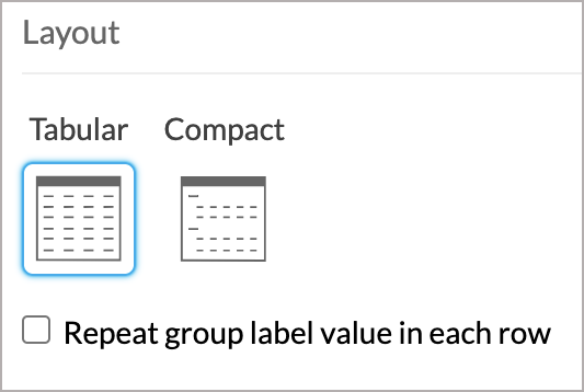
    • Repeat group label value in each row: In case, you wish to repeat the group label for each row, select this checkbox.
      
  • Compact Layout: This is a close-packed view of the Pivot Table where the rows dropped in the 'Rows' shelf will be grouped and arranged in a single column in your Pivot Table.
    • Indent Level: You can change the indent spacing of the data displayed by choosing an Indent Level. By default, level 1 indent will be applied.
      

To learn more about Tabular and Compact layout, refer to the next section.

• Display: This helps you specify what and how data needs to be displayed in the Pivot Table.

  • Hide row numbers: You can choose to hide the row numbers displayed in the Pivot Table by selecting this checkbox. By default, this will not be selected.

  • Wrap text in Column Headings: You can wrap lengthy column headers by selecting this checkbox.

  • Set default column width to: You can uniformly resize the columns by selecting this checkbox. Once selected, specify the required width (in pixel) in the provided field.
    When this option is selected, Apply to manually resized columns prompt will be displayed. You can choose to apply this new width to the already resized columns by selecting this checkbox.

  • Show Expand/Collapse Icons: You can choose to show/hide the Expand/Collapse (+/-) icons by selecting/unselecting the check-box. By default, the+/- icons will be displayed inline with the cell name when you perform the Expand/Collapse operation on your Pivot Table. To learn more about this option, refer to Working with Pivot Table document.

  • Display 'Unknown' value as: You can specify a value that needs to be displayed in the place of null or empty values present in the underlying data of the pivot. By default, -No Value-  will be displayed here.

Tabular and Compact Layout

Zoho Advanced Analytics allows you to visualize your Pivot Table in two layouts. The difference between the two layouts is the structure, i.e., the way in which the columns dropped in the Rows shelf are arranged in the Pivot Table. You can choose between the below two layouts:

• Tabular Layout
• Compact Layout

Tabular Layout (Default Layout) 
The Tabular Layout is the default layout of your Pivot Table where the columns dropped in the Rowsshelf will be arranged as separate columns in the Pivot Table.

Compact Layout 
The Compact Layout is a close-packed view of the Pivot Table where the rows dropped in the Rowsshelf will be grouped and arranged in a single column in your Pivot Table.

The columns dropped in the Rows shelf will be grouped and arranged in a single column with Row Labels as the column name. You can later change this column name by clicking the Edit icon that appears on mouse hover.

Show/Hide

You can choose to hide columns and display only the required columns in a Pivot View using theShow/Hide option.

Show/Hide Columns

When you create a Pivot View in Zoho Advanced Analytics app, all the columns will be displayed by default. You can choose to show/hide the required columns in Zoho Advanced Analytics. To do this:

1. Open the Pivot View.
2. Click the Show/Hide option in the toolbar or right-click the required cell and select Show/Hide Columns. Click either of the below values:
   • Hide <Column Name>: This option is used to hide the selected column.
   • Hide All <Column Name>: This option will be available if you have repetitive columns. Using this option will hide all the columns with the same column name.

Alternatively, you can click the Show/Hide option in the toolbar or right-click the required cell and select Show/Hide Columns > More... option.
​

The Show/Hide Columns dialog will appear, listing all the columns available on your Pivot. You can choose to hide columns by disabling the checkbox inline to the column name.
​

Show/Hide Totals

In the Zoho Advanced Analytics, by default, sub-totals of individual columns, and the grand total of all the rows and columns get automatically added and shown as part of the Pivot Table. Zoho Advanced Analytics also allows you to turn off these totals when they are not required, or to change the totals' positions.

Follow the steps below to customize the sub-totals and the grand-totals in your pivot.

1. Open the Pivot Table.
2. Click the Show/Hide option in the toolbar or right-click the corresponding cell/column in the pivot table and select Show/Hide Totals > More... menu option
3. The Show/Hide Total dialog will open with the following options.
   

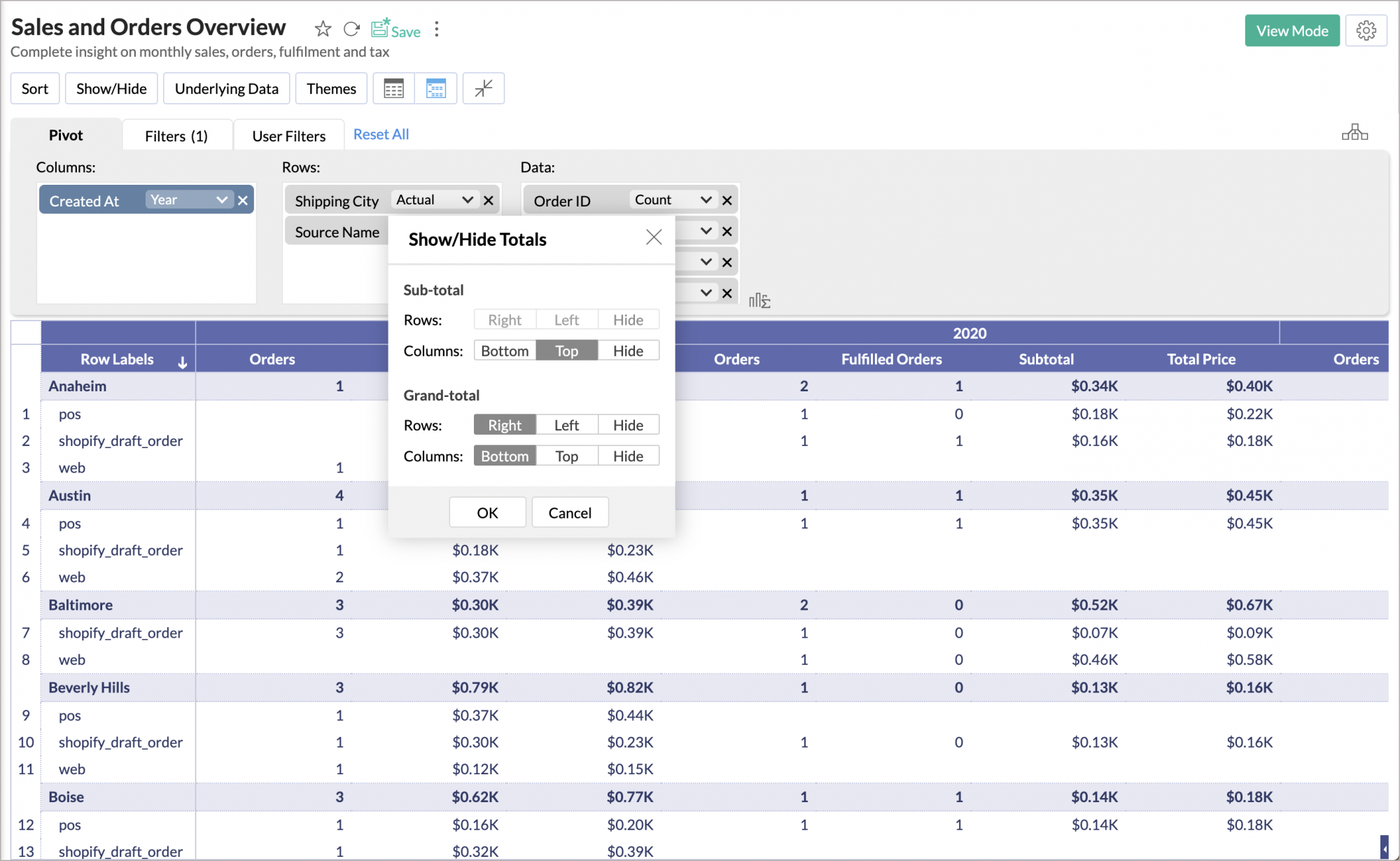
• Sub-total - This lists the option to show or hide the Row and the column sub-totals. 
  • Rows - Select Right or Left to display the sub-total in the corresponding position. You can also choose to hide the row sub-total by selecting Hide.
  • Columns - Select Bottom or Top to display the sub-total in the corresponding position. You can also choose to hide the column sub-total by selecting Hide.
• Grand-total - This lists the option to show or hide the Row and the column grand-totals. 
  • Rows - Select Right or Left to display the Grand-total in the corresponding position. You can also choose to hide the row Grand-total by selecting Hide.
  • Columns - Select Bottom or Top to display the Grand-total in the corresponding position. You can also choose to hide the column Grand-total by selecting.

Show Total As

In the Zoho Advanced Analytics by default, the summary function used to display the subtotals and the grand total will be the same as that of the summary function applied to the corresponding data column. You can customize this and apply other summary functions such as sum, average, min, and max on the sub-total that is displayed.

To change this,

1. Right-click anywhere on the Pivot table
2. Select Show Total As and then, select the function that you wish to apply.

In our example, we have applied the average function. Shown below is the Pivot with the Averagefunction applied to the Subtotal and Grand Total.

Please do note that the Show Total As feature is customizable for each data column.

Sorting a Pivot Table

In the Zoho Advanced Analytics, by default, a pivot table data will be sorted in ascending order by the values of the columns from the source table that you assign to Row orientation in a Pivot Table. Zoho Advanced Analytics allows you to change this default sort order in lot of different ways. Below is a brief description of various ways to sort a Pivot Table.

Sorting a Pivot column by its values (by the values of the columns in Row shelf): This option allows you to sort Pivot Table column data in ascending or descending order by its actual values.

To sort a pivot table by its column values:

1. Right-click the column header or on any cell of the corresponding pivot table column whose values has to be sorted.
2. In the pop-up menu, select the required sort order and then By Column (column specific) option.

For example if a pivot table has Product category and Productcolumns in Row shelf (Row Orientation), initially the Product Categories and Products will be ordered alphabetically in ascending order. 

Sorting a Pivot Table column by its corresponding data values(by values of the column in Data shelf): This option allows you to sort Pivot Table columns based on data values corresponding to each pivot column value.

To sort a pivot table based on its data values:

1. Right-click the data value column header or on any data value cell corresponding to a Pivot Table column based on which you want to sort summary values.
2. In the pop-up menu, select the required sort order.

Sorting Pivot Table columns by its corresponding summary values: This option allows you to sort Pivot Table columns based on summary values corresponding to pivot column values.

To sort a pivot table based on its summary values:

1. Right-click the summary column's header.
2. In the pop-up menu, select the required sort order and then select the column based on which you want to sort summary values.

You can also sort rows by column values by clicking on the arrow icon() at the heading of the corresponding column. A down arrow indicates that the column is sorted in ascending order. An up arrow indicates the column is sorted in descending order.

Conditional Formatting

Conditional formatting feature allows you to visually highlight data cells in a pivot table with different styles based on matching conditions. You have to specify the required conditions/criteria for formatting. When data in a cell meets the condition, the Zoho Advanced Analytics applies the corresponding formatting style that you have specified to the specific cell.   

To apply conditional formatting:

1. Open the Pivot Table for which you want to apply Conditional Formatting.  
2. Right-click on any one of the cells in the data series for which you want to apply conditional formatting.  
3. In the menu, click Conditional Formatting.
4. The Conditional Formatting dialog opens with options for specifying the conditions and selecting colors for font and background. You can also insert texts and icons using the Additional Formatting Options dialog to highlight your condition.
5. Click the drop-down arrow under Condition header and select the type of the condition that you want to apply.
6. Type the matching value that you want to use for the condition in the Value text box.
7. Select the required colors for the font and background.
   
8. Click the  icon to add text and icons.
9. You can add any number of conditions using +Add Condition link.
10. Conditions specified will be evaluated from top to bottom and the corresponding formatting options will be applied on the data cell that meets the condition.   
11. Click OK after you have added all the conditions.
12. You can also view and modify all the conditional formats applied over the pivot in the Conditional Format tab in Settings section.   
    

Applying Themes

Zoho Advanced Analytics allows you to customize the look and feel of your Pivot table using colorful and attractive themes. You can customize your Pivot Table using the options provided to suit your taste. Please do note that this option is available only as a part of the new charting library that was released recently.

Read the below steps to learn about changing the Pivot Theme.

1. Open the Pivot Table
2. Click the Themes button. The Themes dialog will open as shown below.
   
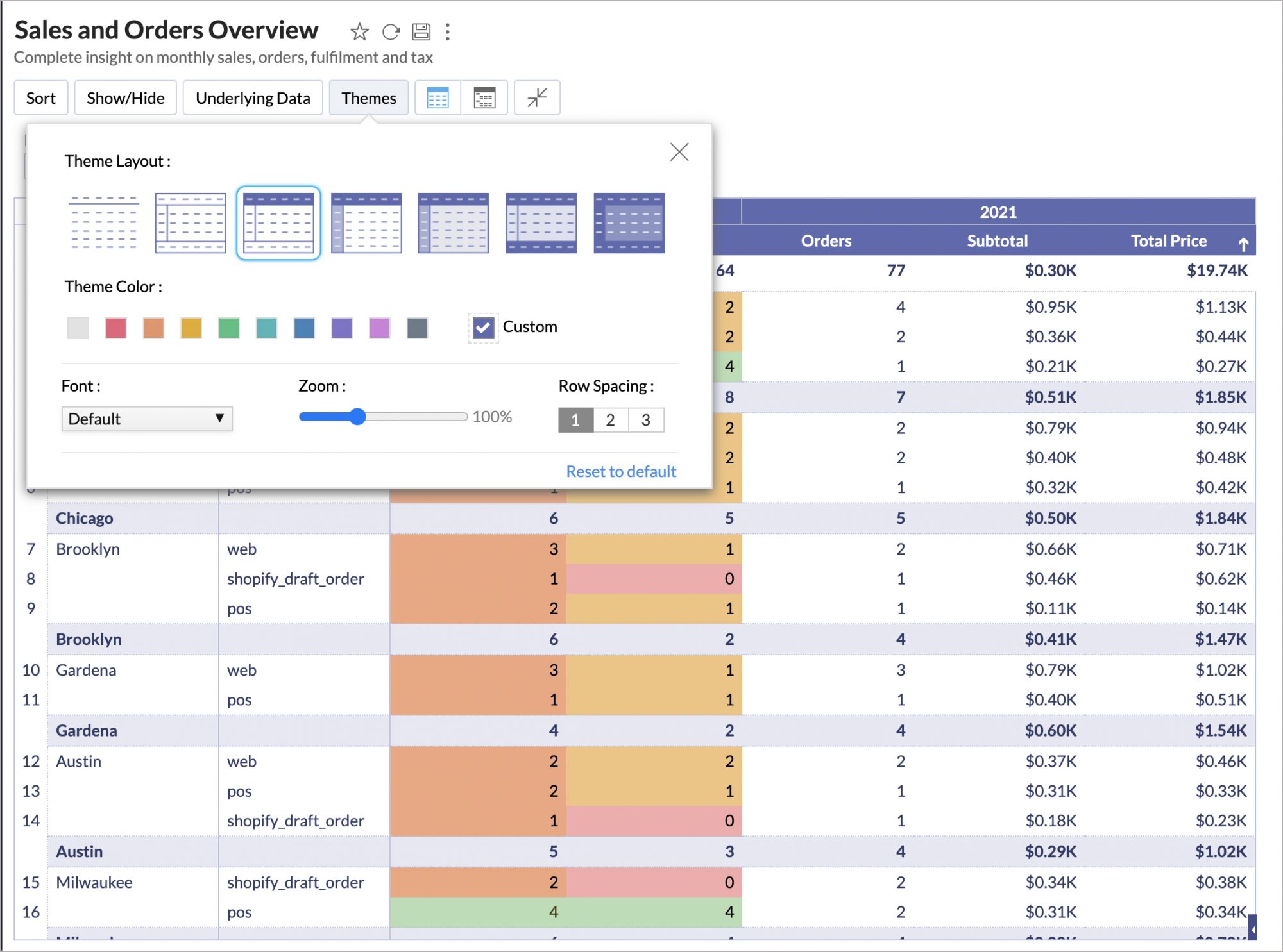
3. You can select an appropriate theme to suit your needs and customize it using the options available. The Themes dialog allows you to select the,
   • Theme Layout: You can choose a layout from the available set of seven layouts.
   • Theme Color: Select a color that you wish to apply.
   • Font: Select the font for the text in your Pivot.
   • Zoom: You can Zoom in or Zoom out. This will increase or decrease the size of your Pivot Table.
   • Row spacing: You can alter the row spacing using the predefined options available.
4. As you choose the themes, the changes will be dynamically applied in the background.
5. If you wish to undo the changes click Reset.
6. If you want to reset the theme to the default theme click the Reset to default option.
7. Save the Pivot Table.